European
Driven by the smile at one expiry.
No model needed: read the arbitrage-free implied surface; a model only interpolates it.
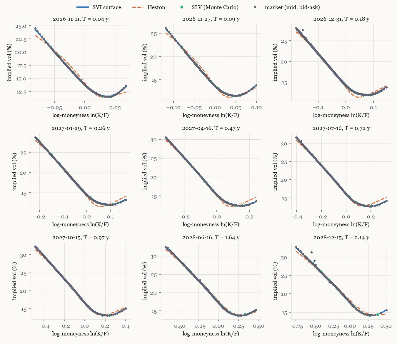
Gatheral (2004); Gatheral and Jacquier (2014). Here: SVI fit within 4 to 10 bp.
Price vanilla and exotic options, watch the Monte Carlo diffuse, and see how much the model matters once the smile is fixed: Heston, local volatility and a stochastic-local-volatility model, all calibrated to the SPX.
Code on GitHub Calibration and methods
Spot 100, Black-Scholes pricers with their Greeks. The Monte Carlo below can switch to the Heston dynamics calibrated on SPX. Everything runs in your browser.
Once the vanillas are fitted, what still differs between models is the dynamics. The product decides how much that matters.
Driven by the smile at one expiry.
No model needed: read the arbitrage-free implied surface; a model only interpolates it.
Gatheral (2004); Gatheral and Jacquier (2014). Here: SVI fit within 4 to 10 bp.
Driven by early exercise, rates and dividends.
Tree or PDE on local vol for one factor; Longstaff-Schwartz once the model has more.
Cox, Ross and Rubinstein (1979); Longstaff and Schwartz (2001). Here: both, cross-checked.
Averaging damps the path: mostly the term structure of vol.
Local vol is usually enough; the geometric Asian is a near-perfect control variate.
Kemna and Vorst (1990); Lévy (1992). Here: the four models agree within 1.2 %.
Driven by the spot-vol dynamics and the forward skew, not just today's smile.
Stochastic-local vol: the leverage fits the smile, the vol of vol sets the dynamics.
Lipton (2002); Ren, Madan and Qian (2007); Guyon and Henry-Labordère (2012). Here: the up-and-out call ranges from 3.5 to 4.7.
Forward-start options and cliquets live on the forward smile; variance swaps on the whole strip.
Stochastic vol or SLV for cliquets; static replication for variance swaps.
Bergomi (2016); Demeterfi, Derman, Kamal and Zou (1999).
Four models calibrated to the same SPX smile (spot rescaled to 100), one-year products, priced by Monte Carlo in the Python library. Each dot is a model; prices are shown relative to the SLV model.
In the SLV model the mixing fraction moves from pure local vol (0) to the full calibrated Heston vol of vol (1). Each point has its own leverage calibration: the vanillas stay on the market while the barriers move. At 1 the leverage no longer fits the at-the-money vol (44 bp off), so that point is not a valid calibration.
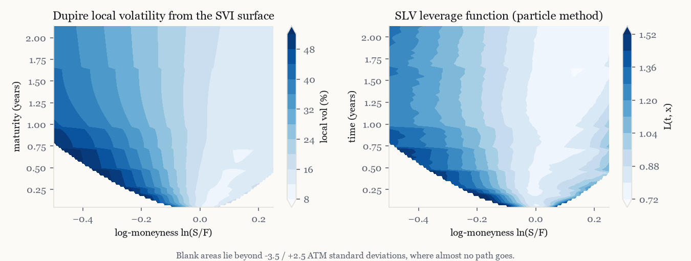
Snapshot of 27 October 2026, 13:37 New York, 9 expiries from two weeks to two years, 1,694 out-of-the-money quotes. Discount factors and forwards from put-call parity. Three steps: the implied surface, Heston on the same quotes, then the SLV leverage by particles. Errors in basis points of implied vol; local vol and SLV are repriced by Monte Carlo (300,000 paths, standard error 3 to 4 bp) against the surface they are built on.